1. Statistics learned with Python 2-1. Probability distribution [discrete variable]
- ** Discrete random variable ** is a variable that takes discrete values like a dice, for example, "1" is followed by "2", "2" is followed by "3", and so on. In the meantime, there are no continuous numbers such as 1.1, 1.2, 1.3, ..., 1.8, 1.9.
- We will look at the characteristics of the main ** discrete probability distributions ** using
pmf(probability mass function) andrvs(random variates) of scipy.stats. I will.
#Import Numerical Library
import numpy as np
import scipy as sp
import pandas as pd
from pandas import Series, DataFrame
#Import visualization library
import matplotlib.pyplot as plt
import matplotlib as mpl
import seaborn as sns
%matplotlib inline
#Japanese display module of matplotlib
!pip install japanize-matplotlib
import japanize_matplotlib
⑴ Bernoulli distribution
- The occurrence of either of the only two types of events is called the ** Bernoulli trial **.
- ** Bernoulli distribution ** is the probability distribution that each event occurs in one Bernoulli trial.
- For example, if you throw a coin 8 times and the front side comes out, it will be 0, and if the back side comes out, it will be 1 and the result is assumed as follows.
x = np.array([0,0,1,1,0,1,0,0])

#Calculate the probability distribution
p = len(x[x==1]) / len(x)
pmf_bernoulli = sp.stats.bernoulli.pmf(x, p)

#Visualization
plt.vlines(x, 0, pmf_bernoulli,
           colors='blue', lw=50)
plt.xticks([0,1])
plt.xlim([0 - 0.5, 1 + 0.5])
plt.grid(True)
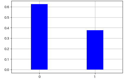
| Two types of events | probability |
|---|---|
| 0 | 0.625 |
| 1 | 0.375 |
⑵ Binomial distribution
- The probability distribution of how many times an event occurs when Bernoulli trials that are independent of each other are repeated n times is called the ** binomial distribution **.
- For example, use
binom.pmfto find the probability that a coin with a probability p of 50% will appear 5 times and 2 of them will appear.
sp.stats.binom.pmf(n=5, p=0.5, k=2)

- Assuming that the trial of throwing a coin with a probability p of 20% to appear 10 times and counting the number of times the table appears was repeated 10,000 times, use
binom.rvsto generate a pseudo-random number that follows a binomial distribution. To do. - Furthermore, using
binom.pmf, calculate the probability distribution of the number of times the table appears when a coin with a probability p of 20% appears 10 times, and compare it with the histogram of pseudo-random numbers.
#Generate pseudo-random numbers
np.random.seed(1)
rvs_binom = sp.stats.binom.rvs(n=10, p=0.2, size=10000)

#Get the probability distribution
m = np.arange(0, 10+1, 1)
pmf_binom = sp.stats.binom.pmf(n=10, p=0.2, k=m)

#Visualization
sns.distplot(rvs_binom, bins=m,
             kde=False, norm_hist=True, label='rvs')
plt.plot(m, pmf_binom, label='pmf')
plt.xticks(m)
plt.legend()
plt.grid()
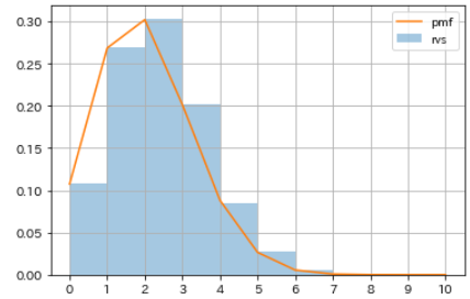
| Number of times the table appears | probability |
|---|---|
| 0 | 0.107374182 |
| 1 | 0.268435456 |
| 2 | 0.301989888 |
| 3 | 0.201326592 |
| 4 | 0.088080384 |
| 5 | 0.026424115 |
| 6 | 0.005505024 |
| 7 | 0.000786432 |
| 8 | 0.000073728 |
| 9 | 0.000004096 |
| 10 | 0.000000102 |
⑶ Poisson distribution
- The probability of a very rare event, such as the number of raindrops per unit area or the number of accidents that occur at an intersection in a year, follows the ** Poisson distribution **.
- In other words, it is a probability distribution that occurs at a constant rate for a certain time or area, and the number of samples n is sufficiently large and the probability p is very small.
- For example, use
poisson.pmfto find the probability that an average of 5 occurrences will occur only 2 times in a given period.
sp.stats.poisson.pmf(k=2, mu=5)

- The parameter of the Poisson distribution is the ** average number of occurrences mu ** of an event, which is also called ** intensity ** or ** λ (lambda) **.
- Assuming that the probability p of an event occurring is 20% and the number of times it has occurred is repeated 10,000 times,
poisson.rvsis used to generate a pseudo-random number that follows a Poisson distribution. - Furthermore, using
poisson.pmf, calculate the probability distribution when the probability of occurrence p is 20%, and compare it with the histogram of pseudo-random numbers.
#Generate pseudo-random numbers
np.random.seed(1)
rvs_poisson = sp.stats.poisson.rvs(mu=2, size=10000)

#Get the probability distribution
m = np.arange(0, 10+1, 1)
pmf_poisson = sp.stats.poisson.pmf(mu=2, k=m)

#Visualization
sns.distplot(rvs_poisson, bins=m,
             kde=False, norm_hist=True, label='rvs')
plt.plot(m, pmf_poisson, label='pmf')
plt.xticks(m)
plt.legend()
plt.grid()
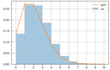
| Number of occurrences | probability |
|---|---|
| 0 | 0.135335283 |
| 1 | 0.270670566 |
| 2 | 0.270670566 |
| 3 | 0.180447044 |
| 4 | 0.090223522 |
| 5 | 0.036089409 |
| 6 | 0.012029803 |
| 7 | 0.003437087 |
| 8 | 0.000859272 |
| 9 | 0.000190949 |
| 10 | 0.000038190 |
- Now consider the relationship between the ** Poisson distribution ** and the ** binomial distribution **.
- Calculate the probability distribution of ** binomial distribution ** when the number of trials n is large enough and the probability p is very small, and compare it with the previous example of ** Poisson distribution **.
#Specify parameters
n = 100000000
p = 0.00000002

#Calculate the probability distribution of the binomial distribution
num = np.arange(0, 10+1, 1)
pmf_binom_2 = sp.stats.binom.pmf(n=n, p=p, k=num)

#Visualization
plt.plot(m, pmf_poisson,
         color='lightgray', lw=10, label='poisson')
plt.plot(m, pmf_binom_2,
         color='black', linestyle='dotted', label='binomial')
plt.xticks(num)
plt.legend()
plt.grid()
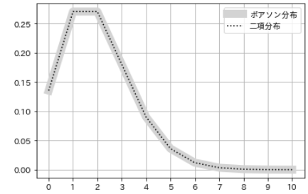
- In this case, the ** Poisson distribution ** and the ** binomial distribution ** are almost the same, indicating that they are closely related.
- ** Poisson distribution ** approximates the situation when the probability p of occurrence of ** binomial distribution ** is very small and the number of trials n is sufficiently large.
⑷ Geometric distribution
- When repeating independent Bernoulli trials with a success probability of p, the probability distribution ** followed by the number of trials k until the first success is called the ** geometric distribution **.
- For example, use
geom.pmfin scipy.stats to get the probability of throwing a dice only once and getting a" 1 ".
%precision 3
sp.stats.geom.pmf(k=1, p=1/6)

- There are 6 dice in all, and if all have the same probability, 1/6 is 0.167, of course.
- Throw one after another and find the probability that "1" will appear for the first time in the second time, the probability that "1" will appear for the first time in the third time, ..., and the probability that "1" will appear for the first time in the 10th time.
#Specify the number of trials
num = np.arange(1, 11, 1)

#Calculate the probability distribution
prob = []
for i in num:
    value = sp.stats.geom.pmf(k=i, p=1/6)
    prob.append(value)

#Visualization
plt.bar(num, prob)
plt.xticks(num)
plt.xlabel('Number of times until 1 appears for the first time')
plt.ylabel('probability')
plt.show()
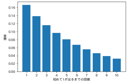
- The probability of throwing k times, failing up to the k-1th time, and succeeding for the first time at the kth time, so the probability distribution in this case is as follows.
| Number of trials | probability | a formula |
|---|---|---|
| 1 | 0.167 | ⅙ |
| 2 | 0.139 | ⅚ ・ ⅙ |
| 3 | 0.116 | ⅚ ・ ⅚ ・ ⅙ |
| 4 | 0.096 | ⅚ ・ ⅚ ・ ⅚ ・ ⅙ |
| 5 | 0.080 | ⅚ ・ ⅚ ・ ⅚ ・ ⅚ ・ ⅙ |
| 6 | 0.067 | ⅚ ・ ⅚ ・ ⅚ ・ ⅚ ・ ⅚ ・ ⅙ |
| 7 | 0.056 | ⅚ ・ ⅚ ・ ⅚ ・ ⅚ ・ ⅚ ・ ⅚ ・ ⅙ |
| 8 | 0.047 | ⅚ ・ ⅚ ・ ⅚ ・ ⅚ ・ ⅚ ・ ⅚ ・ ⅚ ・ ⅙ |
| 9 | 0.039 | ⅚ ・ ⅚ ・ ⅚ ・ ⅚ ・ ⅚ ・ ⅚ ・ ⅚ ・ ⅚ ・ ⅙ |
| 10 | 0.032 | ⅚ ・ ⅚ ・ ⅚ ・ ⅚ ・ ⅚ ・ ⅚ ・ ⅚ ・ ⅚ ・ ⅚ ・ ⅙ |
⑸ Discrete uniform distribution
- There are two types of uniform distribution, discrete type and continuous type. The uniform distribution with discrete random variables is called ** discrete uniform distribution **.
- A distribution with equal probabilities for all events, for example dice follow a ** discrete uniform distribution ** because all dice have equal probabilities of rolling 1 to 6.
#Specify all events
num = np.arange(1, 7, 1)

#Calculate the probability distribution
prob = []
for i in num:
    value = 1 / len(num)
    prob.append(value)

#Visualization
plt.bar(num, prob)
plt.xticks(num)
plt.xlabel('Dice roll')
plt.ylabel('probability')
plt.show()
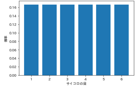
| Dice roll | probability |
|---|---|
| 1 | 0.167 |
| 2 | 0.167 |
| 3 | 0.167 |
| 4 | 0.167 |
| 5 | 0.167 |
| 6 | 0.167 |
⑹ hypergeometric distribution
- For example, suppose you have a total of 20 lots, 7 of which are winning. How many hits will you get when you randomly select 12 out of 20?
- The distribution with this "number to be assigned" as a random variable is called ** hypergeometric distribution **.
- There are three parameters, which are the total number M, the number n per, and the number N to be selected.
#Specify parameters
M = 20 #Total number
n = 7  #Number of hits
N = 12 #Number of selections

#Create a random variable
k = np.arange(0, n+1)

#Create a model
hgeom = sp.stats.hypergeom(M, n, N)
#Calculate the probability distribution
pmf_hgeom = hgeom.pmf(k)

#Visualization
plt.bar(k, pmf_hgeom)
plt.xticks(k)
plt.xlabel('Number of hits')
plt.ylabel('probability')
plt.show()
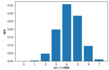
| Number of hits | probability |
|---|---|
| 0 | 0.00010 |
| 1 | 0.00433 |
| 2 | 0.04768 |
| 3 | 0.19866 |
| 4 | 0.35759 |
| 5 | 0.28607 |
| 6 | 0.09536 |
| 7 | 0.01022 |
⑺ Negative binomial distribution
- ** Negative binomial distribution ** finds the probability of success k times in n trials, provided that the last trial is successful.
- In the binomial distribution, the number of successes k is a random variable, but in the ** negative binomial distribution **, the number of successes k is fixed. ** For random variables, use the number of failures n-k ** instead of the number of trials n.
- For example, how many times do you need to flip a coin toss before it comes out three times? In other words, the random variable is the number of failures, which is how many times it must fail before it succeeds three times.
#Specify parameters
N = 12  #Number of trials
p = 0.5 #Probability of success
k = 3   #Number of successes

#Calculate the probability distribution
pmf_nbinom = sp.stats.nbinom.pmf(range(N), k, p)

#Visualization
plt.bar(range(N), pmf_nbinom)
plt.xlabel('Number of failures')
plt.ylabel('probability')
plt.xticks(range(N))
plt.show()
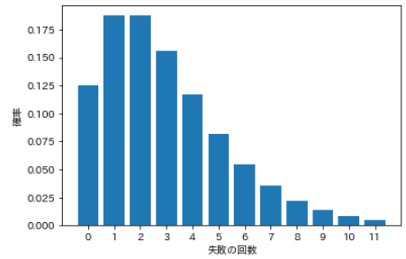
| Number of failures | probability |
|---|---|
| 0 | 0.125 |
| 1 | 0.188 |
| 2 | 0.188 |
| 3 | 0.156 |
| 4 | 0.117 |
| 5 | 0.082 |
| 6 | 0.055 |
| 7 | 0.035 |
| 8 | 0.022 |
| 9 | 0.013 |
| 10 | 0.008 |
| 11 | 0.005 |
Summary
We have looked at the discrete probability distribution, but we will summarize it in a list with an awareness of what is a random variable and, in a nutshell, what to put on the x-axis.
| Types of probability distributions | Random variable | Parameters | |
|---|---|---|---|
| ⑴ | Bernoulli distribution | Event 0, 1 | Probability of occurrence p |
| ⑵ | Binomial distribution | Number of trials | Probability of occurrence p,Number of occurrences k,Number of trials n |
| ⑶ | Poisson distribution | Number of trials | Average number of occurrences mu |
| ⑷ | Geometric distribution | Number of trials | Probability of success p,Number of trials k |
| ⑸ | Discrete uniform distribution | Event type | ※scipy.Uniform distribution of atats is continuous only |
| ⑹ | Hypergeometric distribution | Number of successes | Total number M,Number of successes in the whole n,Number of selections N |
| ⑺ | Negative binomial distribution | Number of failures | Probability of success p,Number of successes k,Number of trials N |
Recommended Posts